In financial applications a simple moving average (SMA) is the unweighted (or equally weighted) mean of the previous n datum points.
An example of a simple equally weighted running mean for a n-day sample of closing price is the mean of the previous n days’ closing prices. If those prices are  then the formula is
When calculating successive values, a new value comes into the sum and an old value drops out, meaning a full summation each time is unnecessary for this simple case,
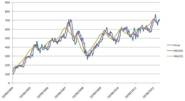
Following graph depicts the Moving Average of Google Weekly closing price for 8 years for window size 10 & 25
Below is an another example of a 5-day moving average evolving over three days
Daily Closing Prices: 9,10,11,12,13,14,15
First day of 5-day SMA:  (9+10+11 + 12 + 13 ) / 5 = 11
Second day of 5-day SMA:  (10+11+12 + 13 + 14 ) / 5 = 12
Third day of 5-day SMA:  (11+12+13 + 14 + 15 ) / 5 = 13
Moving average in q
KDB have a built-in function mavg to find the simple moving average :
q)5 mavg 9 + til 7
9 9.5 10 10.5 11 12 13
Note in the above example the first 4 averages are the partial average as they use less than 5 terms to compute the average, so we will drop/cut the first 4 results.
In time series analysis, Moving Average at a particular data point is computed using previous N terms, so we can get the Moving average only after N data points.
q)4_5 mavg 9 + til 7
11 12 13f
Source: Wikipedia, StockCharts


