Moving Average

In statistics, a Moving Average is used to analyze a set of data points by creating a series of averages of different subsets of the full data set.

Given a data series and fixed subset size(N), the first element of Moving Average is obtained by averaging the initial fixed subset (first N elements) of number series. Then the subset is move forward by 1 element, removing the first element and adding the N+1^th element of the subset, and average is calculated for the 2^nd element of the Moving average. And the process is repeated over the entire data series.

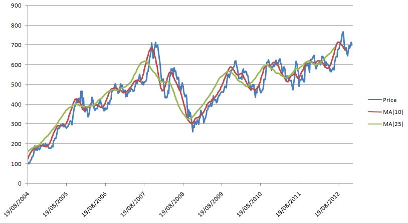
Following graph depicts the Moving Average of Google Weekly closing price for 8 years for window size 10 & 20.

Moving Average is used commonly for analyzing the short term fluctuations from a time series data and highlighting the long term trends. It can be easily seen in the above graph that the line MA(20) is smoothing out a lot of fluctuation as compared to the MA(10).

Moving averages help smooth price action and filter out the noise. They also form the building blocks for many other technical indicators and overlays, such as the McClellan Oscillator and Bollinger Bands.

Types of Moving Average :

• Moving average (SMA)
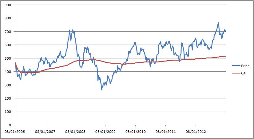
• Cumulative moving average (CMA)
• Weighted moving average
• Exponential moving average (EMA)

Simple moving average (SMA) and Exponential moving average (EMA) are the most popular type of Moving Average.

Moving Average Excel

OHLC (Open-High-Low-Close)

An OHLC chart is typically used to illustrate the Opening , High, Low and Closing price of a security/Instrument during a certain period of time. It displays more information about the price movement as compared to a Line chart.

This type of chart is used by Technical Analysts to spot the trends of security on a short term basis.

Ways of displaying OHLC

• Bar Chart
• Candlestick Chart

Both charts display exactly same information but Candlestick chart is more preferred among traders as it is easier to read.

Bar Chart

Each vertical line on the chart shows the price range (the highest and lowest prices) over a period of time. The open price is marked by a dash pointing to the left and the close price is marked by a dash pointing to the right.

 

 

 

Candlestick Chart

In a candlestick chart the wider bodies of the candles show the opening and closing prices during the period. And the wicks (the lines on top and bottom of the candles) show the lowest and highest prices during the period.

 

 

q Implementation

Since KDB is specially designed for time series data ,there are some built-in functions which makes it trivial to write a query to find OHLC in KDB

q)select open:first price, high:max price, low:min price , close:last price 
by sym,date from quote

q)select open:first price, high:max price, low:min price , close:last price 
by date from quote where sym=`goog

Resources:

• http://en.wikipedia.org/wiki/OHLC
• http://en.tradimo.com/learn-to-trade/
• http://www.highcharts.com

Cumulative Moving Average

A cumulative moving average, computes the running averages of an ordered datum stream.

For example, an investor may want the average price of all of the stock transactions for a particular stock up until the current time. As each new transaction occurs, the average price at the time of the transaction can be calculated for all of the transactions up to that point using the cumulative average, typically an equally weighted average of the sequence of i values x₁, …, x_i up to the current time:

The new cumulative average when a new value x_i+1 arrives can be calculated using the formula:

Following is an example of cumulative moving average of  Google prices.

Cumulative average in q

KDB provides a built in function avgs (running averages) to calculate the cumulative averages.

q)avgs 17 23 44 12 2 36 37 44 28 20
17 20 28 24 19.6 22.33333 24.42857 26.875 27 26.3

If you are Sachin Tendulkar fan then you would be interested to see how he managed to keep CMA of his ODI runs near to 40.

Simple Moving Average

In financial applications a simple moving average (SMA) is the unweighted (or equally weighted) mean of the previous n datum points.

An example of a simple equally weighted running mean for a n-day sample of closing price is the mean of the previous n days’ closing prices. If those prices are then the formula is

When calculating successive values, a new value comes into the sum and an old value drops out, meaning a full summation each time is unnecessary for this simple case,

Following graph depicts the Moving Average of Google Weekly closing price for 8 years for window size 10 & 25

Below is an another example of a 5-day moving average evolving over three days

Daily Closing Prices: 9,10,11,12,13,14,15
First day of 5-day SMA:  (9+10+11 + 12 + 13 ) / 5 = 11
Second day of 5-day SMA:  (10+11+12 + 13 + 14 ) / 5 = 12
Third day of 5-day SMA:  (11+12+13 + 14 + 15 ) / 5 = 13

Moving average in q

KDB have a built-in function mavg to find the simple moving average :

q)5 mavg 9 + til 7
9 9.5 10 10.5 11 12 13

Note in the above example the first 4 averages are the partial average as they use less than 5 terms to compute the average, so we will drop/cut the first 4 results.

In time series analysis, Moving Average at a particular data point is computed using previous N terms, so we can get the Moving average only after N data points.

q)4_5 mavg 9 + til 7
11 12 13f

Source: Wikipedia, StockCharts

Mode

The mode is the value that appears most often in a set of data.

Like the statistical mean and median, the mode is a way of expressing, in a single number, important information about a random variable or a population.

The mode is not necessarily unique, since the same maximum frequency may be attained at different values.

Source: Wikipedia

The mode of a sample is the element that occurs most often in the collection.

For example: Mode of the sample {3, 7, 5, 13, 20, 23, 39, 23, 40, 23, 14, 12, 56, 23, 29} is 23.

It is not necessary that the mode for a given sample is always unique.  There could be multiple modes of the given dataset, if it have 2 modes then we call the dataset as bimodal and if it have more than 2 modes then we call the dataset as multimodal.

bimodal example : {1, 3, 3, 3, 4, 4, 6, 6, 6, 9}  have 2 modes 3 & 6.

There is currently no built in function in q for finding the mode. Lets try writing it, a simple function could be :

q)mode1:{key[d]where max[c]=c:count each value d:group x}
q)mode1  1 2 3 2 4 5 3 5 6 4 3 2
2 3

The above function is simple but we are not utilizing the features which comes automatically with the dictionary datatype in q.

Here is the new definition, which will return all the modes of the input sample:

q)mode:{where max[c]=c:count each d:group x}
q)mode  1 2 3 2 4 5 3 5 6 4 3 2
2 3

Note that the count, max and where works in a different way in case of dictionary. Here “count each” is actually counting the values corresponding to each key and returns a dictionary, max looks up the maximum value of dictionary range and where returns the key for true dictionary range.

The k equivalent of the above mode function is

k)mode:{&:max[c]=c:#:'=:x}