In number theory, a left-truncatable prime is a prime number if the leading (“left”) digit is successively removed, then all resulting numbers are prime.
For example 9137, since 9137, 137, 37 and 7 are all prime.
A right-truncatable prime is a prime which remains prime when the last (“right”) digit is successively removed.
For example 7393, since 7393, 739, 73, 7 are all prime.
There are exactly 4260 decimal left-truncatable primes and 83 right-truncatable primes.
There are 15 primes which are both left-truncatable and right-truncatable. They have been called two-sided primes.
Source: Wikipedia
The number 3797 has an interesting property. Being prime itself, it is possible to continuously remove digits from left to right, and remain prime at each stage: 3797, 797, 97, and 7. Similarly we can work from right to left: 3797, 379, 37, and 3.
Find the sum of the only eleven primes that are both truncatable from left to right and right to left.
NOTE: 2, 3, 5, and 7 are not considered to be truncatable primes.
q/KDB Implementation
To start with, first i have wrote a function which identifies whether a number is prime or not. To speed up the calculation i am maintaining a dictionary which contains the prime numbers. If a number is not present in the dictionary it will return boolean null which is boolean false.
If a given number is divisible by any prime number lesser than that number than that number is not a prime number.
q)primeDict:(2 3 5 7)!(1111b)
q)isPrime:{$[x~1;0b;x~2;1b;0~x mod 2;0b;primeDict[x];1b;x<last key primeDict;0b;
    any 0=(x mod ) each key primeDict;0b;[primeDict[x]:1b;1b]]}
Warm up the dictionary till 1000000
q)isPrime each til 1000000
To check if all numbers in a given list are prime or not.
q)areAllPrimes:{all isPrime distinct x}
To check whether a given number is Right Prime Truncatable & Left Prime Truncatable.
q)rightPrimeTrunc:{$[isPrime x;areAllPrimes {"J"$neg[y] _string x}[x]
     each til count string x;0b]}

q)leftPrimeTrunc:{$[isPrime x;areAllPrimes {"J"$y _string x}[x] each til count string x;0b]}
We’ll abort the operation if any number contains either 0 4 6 or 8. Since 2 is prime number it might happen that in left or right function, 2 is generated in intermediate operation.
q)haveEvens:{any count[x]>x?/:"0468"}
Now check whether a number contains even number otherwise check its left truncatable & right truncatable.
q)bothPrimeTrunc:{$[haveEvens s:string x;:0b;not leftPrimeTrunc x;0b; rightPrimeTrunc x]}

q)where bothPrimeTrunc each til 1000000
2j, 3j, 5j, 7j, 23j, 37j, 53j, 73j, 313j, 317j, 373j, 797j, 3137j, 3797j, 739397j

q)sum 4_2j, 3j, 5j, 7j, 23j, 37j, 53j, 73j, 313j, 317j, 373j, 797j, 3137j, 3797j, 739397j
 748317j


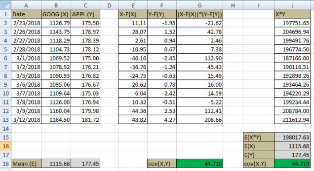
![\operatorname {cov} (X,Y)=\operatorname {E} {{\big [}(X-\operatorname {E} [X])(Y-\operatorname {E} [Y]){\big ]}},](https://wikimedia.org/api/rest_v1/media/math/render/svg/7120384a1c843727d9589e2b33dbc33901d14f42)
 ,
, 
 .
.![\operatorname {Var} (X)=\operatorname {E} \left[(X-\mu )^{2}\right].](https://wikimedia.org/api/rest_v1/media/math/render/svg/55622d2a1cf5e46f2926ab389a8e3438edb53731)
 is random variable & μ is mean of
  )
) 


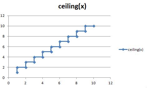
 is the largest integer not greater than x.
 is the smallest integer not less than x.